CFD Course project
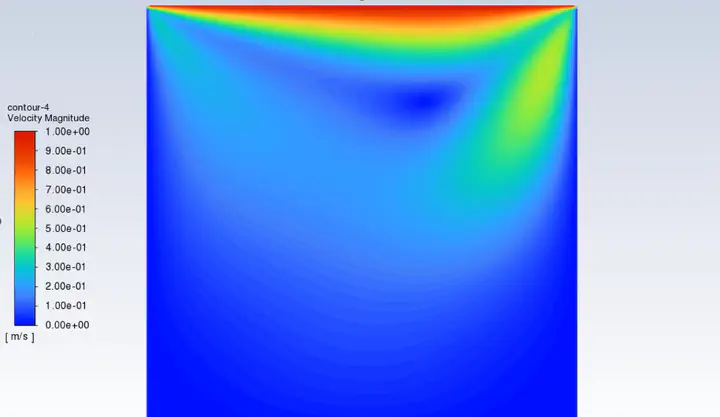 Magnitude veclocity contour of the cavity flow (lid driven flow) illustrated using Ansys Fluent (Image by Kimia Sadafi)
Objective
This project aims to model the flow of fluid inside a rectangular cavity. Method to model the system is to write down equations representing the flow, use finite difference discretization and solving the resulted system of equation to find velocity vector and potential function quantity in each grid node.
To validate the procedure and analysis, a reference paper 1 was used to compare the results and calculate error.
Problem Formulation
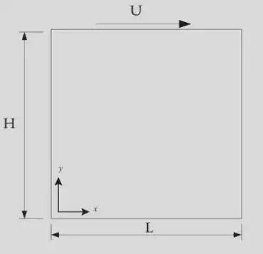
Geometry and Properties
The cavity is a rectangular hole with one moving side (preferably the upper side) and other three sides fixed. The rectangle can be divided into a fine grid for using finite difference approximation. To compare the results with proof paper, we’ve chosen to make a 129 x 129 node grid which is the same as the amount used in the paper.
Length and width of the cavity is chosen to be $1m$, Velocity of upper side is $1 \frac{m}{s}$ and the kinematic viscosity of the fluid is $0.01\frac{m^2}{s}$.
The numbers may seem unrealistic, but since there’s a dimensionless property in fluid dynamic phenomena, we can tune the parameters proportional to each other to make sense out of them, or evaluate the system with its dimensionless properties like Reynolds number. For instance, in this particular example, $Re = 100$.
Equations
To formulate the problem we need to know the equations holding true for the system. In this example equations relating stream function and velocities, equations of vorticity and of course, Navier-Stokes equations are used to model the system.
Stream Function Equations:
$u=\frac{\partial \psi}{\partial y}$ and $v=-\frac{\partial \psi}{\partial x}$
Vorticity Equation:
$\vec{\omega}=\nabla \times \vec{u}$
for a 2D flow, relation between vorticity and stream function is:
$\omega = -(\frac{\partial^2\psi}{\partial x^2} + \frac{\partial^2\psi}{\partial y^2})$
Navier-Stokes Equation:
Assuming incompressible, steady flow we can derive the below equation:
$u\frac{\partial \omega}{\partial x} + v\frac{\partial \omega}{\partial y} = \nu(\frac{\partial^2\omega}{\partial x^2} + \frac{\partial^2\omega}{\partial y^2})$
Boundary Conditions:
All sides of the cavity have no-slip and no-penetration boundary condition, which is essentially equivalent to Neumann boundary condition. It means that velocities perpendicular to the walls are equal to zero, and velocities tangent to the walls are equal to the velocity of the wall itself. If the velocities are defined as $u=u(x,y)$ and $v=v(x,y)$ and length and height of the cavity are $L$ and $H$:
$u(0,y)=v(0,y)=0$
$u(x,0)=v(x,0)=0$
$u(L,y)=v(L,y)=0$
$v(x,H)=0$
$u(x,H)=U$
Above relations will in turn give us value of the vorticity and stream function in boundaries.
Solution
Method to solve this problem is to first discretisize the above equations, then implement a numerical iterative method (Like Jacobi method) to solve system of equations.
Finite Difference Approximation
To discretisize the equations, 2nd order central difference approximation was used.
Stream Function Equation:
$u_{i,j}=\frac{\psi_{i,j+1}-\psi_{i,j-1}}{2\Delta_y}$
$v_{i,j}=\frac{\psi_{i+1,j}-\psi_{i-1,j}}{2\Delta_x}$
Vorticity Equation:
$\frac{\psi_{i+1,j}-2\psi_{i,j}+\psi_{i-1,j}}{\Delta^2_x}+\frac{\psi_{i,j+1}-2\psi_{i,j}+\psi_{i,j-1}}{\Delta^2_y}=-\omega_{i,j}$
Navier-Stokes Equation:
$u_{i,j}\frac{\omega_{i+1,j} - \omega_{i-1,j}}{2\Delta_x}+v_{i,j}\frac{\omega_{i,j+1} - \omega_{i,j-1}}{2\Delta_y}=\nu[\frac{\omega_{i+1,j}-2\omega_{i,j}+\omega{i-1,j}}{2\Delta^2_x}+\frac{\omega_{i,j+1}-2\omega_{i,j}+\omega{i,j-1}}{2\Delta^2_y}]$
Solving Algorithm
As mentioned previously, the method to solve this problem is to use iterative methods. In this example Jacobi method is used and implemented in Matlab. Below is the script used in this project:
Click to view the script
% Numerical Solution For Lid Driven Stream
% Project 1
% Author(s): Kimia Sadafi, Siavash Emami, Amir Mohammad Abbasi

clear; close all; clc;

%% Initialization
itteration = 0;
validation_flag = true;
if validation_flag==true
    V = 0;
    Nx = 129;
    Ny = 129;
else
    V = 1;
    Nx = 101;
    Ny = 101;
end
U = 1;
L = 1;
H = 1;
nu = 0.01;
dx = L/(Nx-1);
dy = H/(Ny-1);
x = linspace(0,L,Nx);
y = linspace(0,H,Ny);
Err_psi = 1;
Err_omega = 1;
beta = dx/dy;
Re = U*L/nu;

u = zeros(Nx,Ny);
v = zeros(Nx,Ny);
psi = zeros(Nx,Ny);
omega = zeros(Nx,Ny);

%% Boundary Conditions
psi(1,:)  = 0;
psi(:,1)  = 0;
psi(Nx,:)  = 0;
psi(:,Ny)  = 0;

v(2:end-1,1) = 0;
v(2:end-1,Ny) = 0;
v(1,2:end-1) = V;
v(Nx,2:end-1) = 0;

u(1,2:end-1) = 0;
u(Nx,2:end-1) = 0;
u(2:end-1,1) = 0;
u(2:end-1,Ny) = U;

%% Calling Funcitons
while(Err_psi > 1e-6 || Err_omega > 1e-6)
    omega(Nx,:) = -2*(psi(Nx-1,:)+v(Nx,:)*dx)/dx^2;
    omega(1,:) = -2*(psi(2,:)+v(1,:)*dx)/dx^2;
    omega(:,Ny) = -2*(psi(:,Ny-1)+u(:,Ny)*dy)/dy^2;
    omega(:,1) = -2*(psi(:,2)+u(:,1)*dy)/dy^2;
    [psi,Err_psi] = Jakobi_psi(Nx,Ny,psi, beta, dx, omega);
    [omega,Err_omega] = Jakobi_omega(Nx,Ny,u,v,beta, dx, omega, nu);

    for i=2:Nx-1
        for j=2:Ny-1
            u(i,j) = (psi(i, j+1) - psi(i, j-1))/(2*dy);
            v(i,j) = (psi(i-1, j) - psi(i+1, j))/(2*dx);
        end
    end
    itteration = itteration+1;
end

vel_mag = sqrt(u.^2+v.^2);
Results
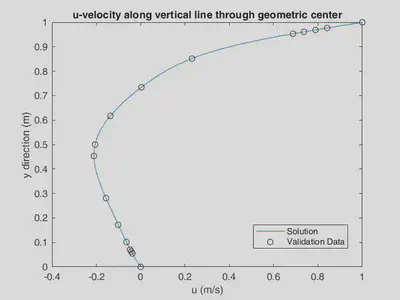
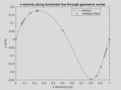
Validation
As mentioned before, we used a paper to proof validity of our solution. In the below figures, it is shown that the calculated velocities are exactly fitted with the proof data from the paper.
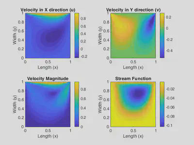
Contours
Also, the contours of velocities in each direction, magnitude velocity and stream function are showed in the figure below:
Ghia, U., Ghia, K. and Shin, C., 1982. High-Re solutions for incompressible flow using the Navier-Stokes equations and a multigrid method. Journal of Computational Physics, 48(3), pp.387-411. ↩︎
Siavash Emami
Mechanical Engineer
My research interests include mobile robots, SLAM and navigation, path planning and control theory.